Gauss Quadrature

It seems to me that many practitioners of finite elements are engineers (myself included), as opposed to mathematicians. Part of the mythos of finite elements is Gauss quadrature. We see its name thrown around when discussing integration in finite elements, and we know that it is an efficient scheme. But us engineers don’t necessarily know what it is, where it comes from, or why it works. I’m going to try to address this gap in knowledge over several few posts — I hope you find these insightful.

Legendre Basis Polynomials

The Legendre polynomials are an orthogonal set of polynomial functions – a useful consequence of this is that they form a linearly independent basis of the polynomials. In other words, any polynomial function can be represented as a linear combination of Legendre polynomials. Let’s walk through an example to demonstrate:

$f(x) = 4x^3 + 3x^2 + 2x + 1$

The normalized (i.e. orthonormal) Legendre polynomials through degree-3 are:

$\mathcal{L}(x) = \left\{ \begin{matrix} 1 \\ x \\ \frac{3}{2}x^2 - \frac{1}{2} \\ \frac{5}{2}x^3 - \frac{3}{2} \end{matrix} \right\}$

Our goal will be to find coefficients, $c_i$ such that $\sum_{i=0}^3 \mathcal{L}_i c_i \equiv g(x) = f(x)$ . To accomplish this, let us define a residual function $r(x) = f(x) - g(x)$ When $r(x) = 0$ then we will know that we have decomposed $f(x)$ into a linear combination of Legendre basis polynomials. We start by trying to find the coefficient for the highest degree term in our residual function. Note that all we need to do in each step is to match the coefficient of the highest-degree monomial term in the residual function with the highest-degree monomial term of the Legendre basis.

Legendre Decomposition Example

Step 1

$\left( \frac{5}{2}x^3 - \frac{3}{2}x \right) c_3 \approx 4x^3 \implies \left( \frac{5}{2}x^3\right) c_3 = 4x^3$

$c_3 = \frac{8}{5}$

Then we update $g(x)$ and $r(x)$

$g(x) = \mathcal{L}_3 c_3 = 4x^3 - \frac{12}{5}x$

$r(x) = 0x^3 + 3x^2 + \frac{22}{5}x +1$ .

Step 2

$\left( \frac{3}{2}x^2 - \frac{1}{2}\right) c_2 = 3x^2 \implies \left( \frac{3}{2}x^2 \right) c_2 = 3x^2$

$c_2 = 2$

Updating $g(x)$ and $r(x)$ :

$g(x) = \mathcal{L}_3 c_3 + \mathcal{L}_2 c_2 = 4x^3 + 3x^2 -\frac{12}{5}x - 1$

$r(x) = 0x^3 + 0x^2 +\frac{22}{5} x + 2$

Step 3

$\left(x\right) c_1 = \frac{22}{5}x$

$c_1 = \frac{22}{5}$

Updating $g(x)$ and $r(x)$ :

$g(x) = \mathcal{L}_3 c_3 + \mathcal{L}_2 c_2 + \mathcal{L}_1 c_1 = 4x^3 + 3x^2 + 2x - 1$

$r(x) = 0x^3 + 0x^2 + 0x + 2$

Step 4

$\left(1\right) c_0 = 2$

$c_0 = 2$

Updating $g(x)$ and $r(x)$ :

$g(x) = \mathcal{L}_3 c_3 + \mathcal{L}_2 c_2 + \mathcal{L}_1 c_1 + \mathcal{L}_0 c_0 = 4x^3 + 3x^2 + 2x +1$

$r(x) = 0x^3 + 0x^2 + 0x + 0$

Result

We can summarize these results in a vector: $\mathbf{c} = \left[ \frac{8}{5}, 2, \frac{22}{5}, 2 \right]^T$

Figure 1: A linear combination of scaled Legendre basis polynomials can represent any polynomial function exactly

The main result of this is to demonstrate that we can decompose any polynomial function into a linear combination of Legendre polynomials. And we can use this property to define the polynomial’s integral in terms of the Legendre polynomials:

$\int f(x) dx = \sum_i \int \mathcal{L}_i c_i \ dx$

All we need to do now is find an efficient means to integrate these basis polynomials (i.e. $\int \mathcal{L}_i c_i \ dx$ . It just so happens that such a means does exist for the Legendre polynomials over the bi-unit domain (i.e. $[-1, 1]$ ). The method we can use to integrate these polynomials is called Gaussian Quadrature, which is a technique that seeks to obtain the best numerical estimate of an integral by picking optimal points at which to evaluate the function, evaluating the function at these optimal points, scaling these function evaluations by scale factors (i.e. weights) associated with each optimal point, and summing the results. Furthermore, the optimal points of an N-point Gaussian quadrature formula are precisely the roots of the orthogonal polynomial for the same interval and weighting function. When the orthogonal polynomials are the Legendre polynomials this is called a Gauss-Legendre scheme. In summary, Gaussian quadrature over the bi-unit domain is:

$\int_{-1}^{1} f(x) \approx \sum_{i}^N f(x_i) \textrm{w}_i$

Building Gauss-Legendre Quadrature Rule

Step 1: Optimal points for integration scheme

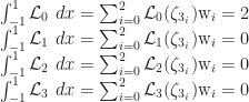
Let’s first investigate how to find the optimal points for a 3-point Gauss-Legendre scheme. We begin by plotting the functions and noticing that over the bi-unit domain every Legendre basis has an integral of $0$ , except for $\mathcal{L}_0$ , which has an integral of $2$ .

Figure 2: Integrals (blue) of the Legendre basis polynomials (black) and the roots (pink) of the polynomials

Step 2: Corresponding scale factors (weights)

Now let’s find the corresponding scale factors (i.e. weights) of the three roots, $\zeta_3$ , of $\mathcal{L}_3$ . First let’s replot the basis functions, this time showing $\mathcal{L}_i$ evaluated at $\zeta_3$ .

Figure 2: Integrals (blue) of the Legendre basis polynomials (black) and the evaluations (green) of each $\mathcal{L}_i$ at the roots of $\mathcal{L}_3$

Figure 2: Integrals (blue) of the Legendre basis polynomials (black) and the evaluations (green) of each $\mathcal{L}_i$ at the roots of $\mathcal{L}_3$

Legendre polynomials evaluated at the roots of $\mathcal{L}_3$

Legendre polynomials evaluated at the roots of $\mathcal{L}_3$

But remember, we know what these integrals should evaluate to:

$\begin{matrix} \int_{-1}^{1}\mathcal{L}_0 \ dx= \sum_{i=0}^2 \mathcal{L}_0(\zeta_{3_{i}})\textrm{w}_i= 2 \\\int_{-1}^{1}\mathcal{L}_1 \ dx= \sum_{i=0}^2 \mathcal{L}_1 (\zeta_{3_{i}})\textrm{w}_i= 0 \\ \int_{-1}^{1}\mathcal{L}_2 \ dx = \sum_{i=0}^2 \mathcal{L}_2 (\zeta_{3_{i}})\textrm{w}_i= 0 \\ \int_{-1}^{1}\mathcal{L}_3 \ dx = \sum_{i=0}^2 \mathcal{L}_3 (\zeta_{3_{i}})\textrm{w}_i= 0 \end{matrix}$

We can encode these conditions in a linear system of equations:

Note that the bottom row is trivial, leading to a more compact system:

Solving this linear system of equations yields:

$\textbf{w} = \left[ \frac{5}{9}, \frac{8}{9}, \frac{5}{9} \right]$

Gaussian Quadrature Example

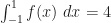
Let’s now try to apply this 3-point Gauss-Legendre scheme to our example function $f(x) = 4x^3 + 3x^2 + 2x + 1$ . We analytically compute the integral so that we can compare results:

Analytic solution

$\int f(x) \ dx = x^4 + x^3 + x^2 + x$

$\int_{-1}^{1} f(x) \ dx = \left[1^4 + 1^3 + 1^2 + 1 \right] - \left[ (-1)^4 + (-1)^3 + (-1)^2 + (-1) \right]$

$\int_{-1}^{1} f(x) \ dx = 4$

Gauss-Legendre

$\int f(x) dx = \sum_i \int \mathcal{L}_i c_i \ dx$

$\int f(x) dx = \sum_{i=0}^3 \left( c_i \sum_{j=0}^2 \mathcal{L}_i(\zeta_{3_{j}}) \textrm{w}_j \right)$

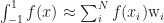
It worked! But this wasn’t example wasn’t exactly true to the fundamental theory of Gaussian quadrature — instead of evaluating the function at the optimal points, we evaluated the Legendre basis polynomials. But here is the key that lets us evaluate the function: Recall that 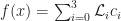$f(x)$ is equivalent to some linear combination of Legendre basis polynomials; $f(x) = \sum_{i=0}^3 \mathcal{L}_i c_i$ . When we evaluate $f(\zeta_{3_0})$ it’s as if we’ve evaluated $\mathcal{L}_i \left(\zeta_{3_0}\right)c_i$ for every value of $i$ . Thus instead of needing to evaluate two nested summations (every Legendre basis evaluated at every optimal point) we only need to evaluate a single summation of $f(x)$ evaluated at each optimal point. Observe:

True Gauss-Legendre Quadrature

$\int f(x) dx = \sum_i f(\zeta_{3_i})\textrm{w}_i$

Figure 3: Gauss quadrature of the Legendre polynomial decomposition (left and right-magenta) is equivalent to
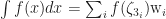
Gauss quadrature of the original function (right-black)

There you have it. A thorough, if a bit pedantic, walkthrough of how Gauss quadrature works. There are some additional points that I didn’t mention, that are important from the perspective of implementing in a finite element code – for both traditional and smooth-spline finite elements. I will try to cover these in a future post.

Legendre Basis Polynomials

Legendre Decomposition Example

Step 1

Step 2

Step 3

Step 4

Result

Building Gauss-Legendre Quadrature Rule

Step 1: Optimal points for integration scheme

Step 2: Corresponding scale factors (weights)

Gaussian Quadrature Example

Analytic solution

Gauss-Legendre

True Gauss-Legendre Quadrature

Share this:

Like this:

Leave a Reply Cancel reply